On December 17, 2025, Starlink satellite 35956 experienced an anomaly. Within a day, SpaceX had partnered with Vantor to photograph the tumbling satellite from orbit using WorldView-3. The image, taken from 241 km away, showed the satellite was “largely intact.”
A comment on LinkedIn caught my attention: How quickly could they take this photo?
I decided to find out.
The Event
The official Starlink announcement reported that satellite 35956 had lost communications and was venting propellant. SpaceX would deorbit it. LeoLabs detected “tens of objects” in the vicinity, though SpaceX described it as a “small number” of trackable debris.
The next day, Michael Nicolls, VP of Starlink Engineering, shared an image:
Imagery collected by Vantor’s WorldView-3 satellite about 1 day after the anomaly shows that @starlink Satellite 35956 is largely intact. The 12-cm resolution image was collected over Alaska from 241 km away. We appreciate the rapid response by @vantortech to provide this… https://t.co/8OcTZsk5Gx pic.twitter.com/1PafjFwuRP
— Michael Nicolls (@michaelnicollsx) December 20, 2025
“Imagery collected by Vantor’s WorldView-3 satellite about 1 day after the anomaly shows that Starlink Satellite 35956 is largely intact. The 12-cm resolution image was collected over Alaska from 241 km away.”
Vantor’s LinkedIn post confirmed the rapid partnership.
This raised a natural question: What determines when two satellites can get close enough for imaging?
Building SatToSat
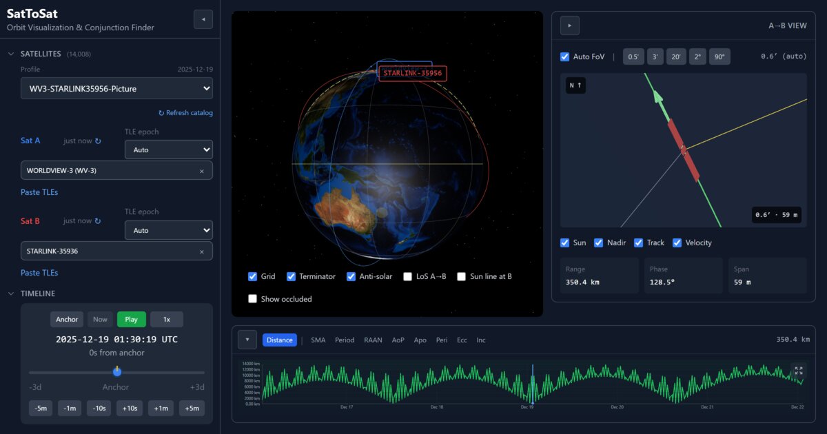
I built SatToSat (repo, live), a tool to explore satellite conjunctions. Given any two satellites, it finds their close approaches over a time window using public Two-Line Element (TLE) data and SGP4 propagation.
This was a “vibe engineered” project - Simon Willison’s term for responsible AI-assisted development, as distinct from Andrej Karpathy’s “vibe coding” where you “forget that the code even exists.” I built it with Claude Code and OpenAI Codex. These AI coding tools have matured significantly over the past few months, and what might have taken weeks of wrestling with Three.js and orbital mechanics libraries came together in days. The iteration cycle of “describe what I want → review generated code and app → refine” has become remarkably productive.
The repository has two parts:
1. Web UI - An interactive 3D visualization for exploring orbits and conjunctions manually. Select any two satellites from the catalog, see their orbital paths, and browse close approaches on a timeline.
2. Analysis Scripts - Python and TypeScript scripts for deeper investigation:
- Conjunction analysis: I implemented the conjunction algorithm in both TypeScript (for the web app) and Python (for verification). Comparing outputs confirmed they match within 27 meters.
- Envelope period analysis: Scripts to analyze the periodic “envelope” pattern of close approaches between satellite pairs (more on this below).
The core conjunction algorithm:
- Load TLEs for both satellites
- Propagate positions at 30-second intervals over ±3 days
- Find local minima in the distance function
- Refine to 100ms precision using ternary search
The Investigation
I attempted to reproduce the reported 241 km approach over Alaska using three different approaches. None succeeded.
Goal 1: Find all close approaches on Dec 17-19
Using public TLE data, I searched for all conjunctions < 1000 km between WorldView-3 and Starlink-35956:
| # | Time (UTC) | Distance | Location |
|---|---|---|---|
| 1 | Dec 17 12:19 | 204 km | Atlantic Ocean (53°N, 17°W) |
| 2 | Dec 19 01:30 | 350 km | Sea of Okhotsk (55°N, 146°E) |
| 3 | Dec 18 23:55 | 981 km | Pacific (47°N, 167°E) |
Result: The closest approach was 204 km on Dec 17 - over the Atlantic, not Alaska. The Dec 19 01:30 UTC conjunction (350 km) is December 18 evening in US time zones, but it’s over the Sea of Okhotsk, not Alaska.
Goal 2: Find approaches over Alaska
I filtered specifically for times when WorldView-3 was over Alaska (including the Aleutian Islands):
| Time (UTC) | Distance | Location |
|---|---|---|
| Dec 18 23:54 | 1,157 km | Western Aleutians (50°N, 168°E) |
Result: The closest approach while over Alaska was 1,157 km - nowhere near 241 km.
Goal 3: Test with post-anomaly TLE
The TLEs from Dec 18 still showed normal orbital parameters. The orbital decay only appeared in a TLE generated on Dec 19 22:47 UTC. I tested by back-propagating this post-anomaly TLE:
| TLE Used | Dec 18 23:55 Distance | Best Approach |
|---|---|---|
| Normal TLEs | 981 km | 204 km (Dec 17) |
| Post-anomaly TLE | 650 km | 190 km (Dec 19 00:42) |
| Reported | 241 km | Alaska |
Result: The post-anomaly TLE improves the Dec 18 distance (650 km vs 981 km), but still doesn’t reproduce 241 km over Alaska.
Summary
| What Was Reported | What I Found |
|---|---|
| 241 km | 204 km (Dec 17) or 350 km (Dec 18 US time) |
| Dec 18 | Dec 17 12:19 UTC or Dec 19 01:30 UTC |
| Over Alaska | Atlantic Ocean or Sea of Okhotsk |
None of the three approaches could reproduce the reported geometry.
What’s Really Going On
Starlink orbital data comes from multiple sources: SpaceX publishes ephemerides to their space-safety portal (updated roughly every 30 minutes) and to Space-Track.org. The 18th Space Defense Squadron also tracks satellites using the Space Surveillance Network. Celestrak’s supplemental GP data is derived from SpaceX’s public ephemerides.
Two possibilities could explain the discrepancy:
Different ephemerides: SpaceX had real-time tracking of their satellite’s actual position—not a smoothed orbital fit from hours ago. The anomaly (tank venting, tumbling) changed the orbit in ways that public TLEs never captured. Even public sources with update cadences measured in minutes to hours may not capture a satellite’s true trajectory during rapid orbital changes. The 241 km approach over Alaska may have existed only in the satellite’s true post-anomaly orbit—one that never appeared in any public data.
A unit transcription error: What if the reported distance was 241 miles, not kilometers? 241 miles converts to 388 km—remarkably close to our 350 km and 383 km approaches on Dec 19. The image could have been captured slightly before or after closest approach. Unit confusion between miles and kilometers has caused problems before (see: Mars Climate Orbiter).
Understanding the “Beat Period”
Back to the original question: How quickly could Vantor take this photo?
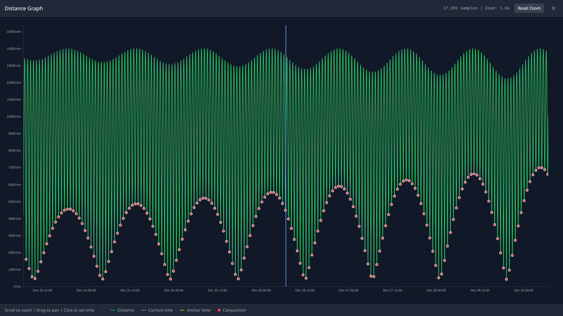
Finding close approaches was straightforward. But while building SatToSat’s distance graph, I noticed something interesting—a clear scalloped pattern emerging in the data. The closest approaches weren’t random; they followed a rhythm.
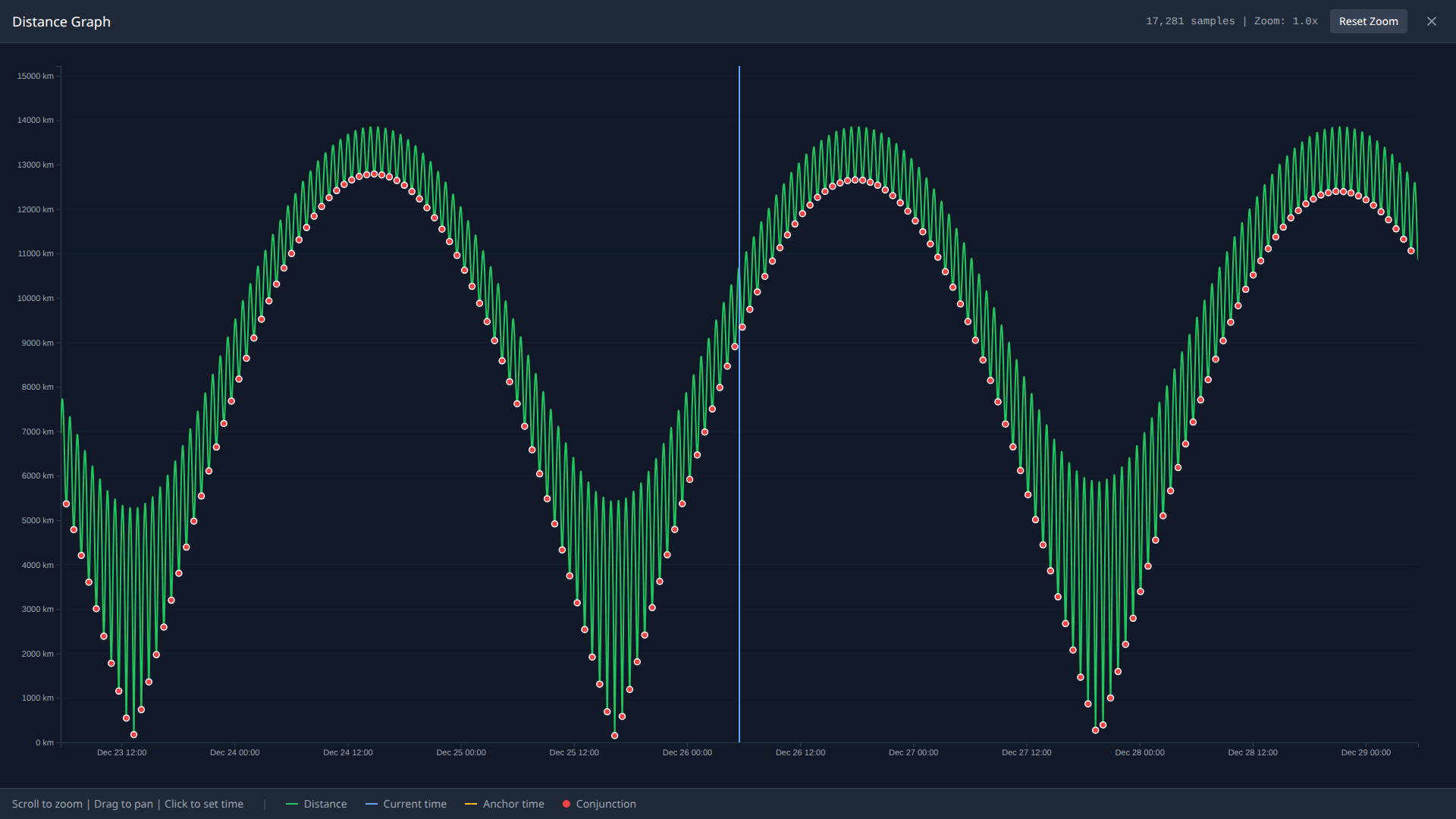
This graph shows the distance between WorldView-3 and a healthy Starlink satellite (Starlink-32153, NORAD 60330) over 6 days. The pattern is unmistakable:
- Close approaches occur roughly every 47 minutes (half the orbital period)
- But the closest approaches repeat every ~51 hours
This “envelope period” - the time between the deepest dips - is what matters for imaging. You might get 8 close approaches within 6 hours, but only one of those will be close enough.
The Physics
The envelope period follows the synodic period formula:
$$T_{envelope} \approx \frac{T_a \times T_b}{|T_a - T_b|}$$Where $T_a$ and $T_b$ are the orbital periods. For WorldView-3 (~97 min) and a healthy Starlink (~94 min), this gives ~51 hours.
Satellites in similar orbits have long envelope periods - the tiny speed difference means it takes days for one to “lap” the other. Different inclinations or altitudes create shorter periods.
| Pair Type | Envelope Period | Why |
|---|---|---|
| Sun-sync vs LEO (WV3-Starlink) | ~51 hrs | 45° inclination difference |
| Same constellation | Never close | Identical orbital planes |
| ISS vs NOAA-20 | ~18 hrs | 47° inclination difference |
An Interesting Detail
On December 17 around 17:32 UTC, WorldView-3 performed an orbital adjustment - raising its altitude by 2.7 km and reducing eccentricity by 67% (a circularization burn). This decreased the beat period with Starlink by about 4 hours.
Was this routine station-keeping, or something else? Without Maxar’s operational logs, I can’t say.
What This Means
For the Starlink-35956 imaging:
The ~1-day timeline was achievable. With a ~42-hour envelope period (shorter due to the anomalous satellite’s lower altitude), a close approach would occur within about 1 day 18 hours of any given moment—well within the reported timeline.
Public TLE data has limits. During satellite anomalies, TLEs lag reality by hours to days. The 110 km discrepancy isn’t a calculation error - it’s a data accuracy problem.
Internal tracking is essential. SpaceX knew the actual orbit; I was working with yesterday’s data.
SatToSat: The Tool
Beyond this investigation, SatToSat is useful for exploring satellite conjunctions generally:
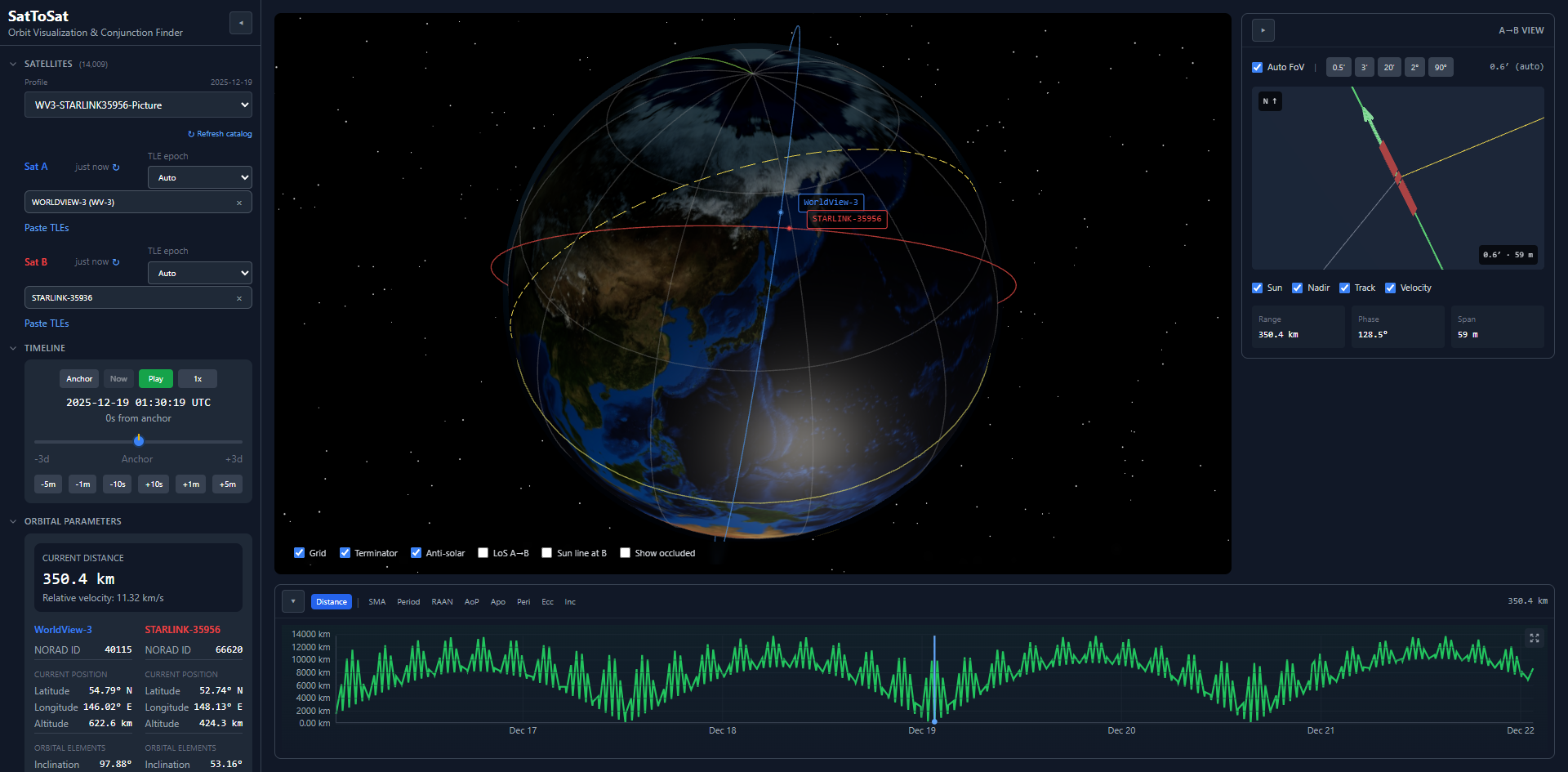
- Select any two satellites from the catalog (~14,000 tracked objects)
- Visualize close approaches on a 3D globe with orbital paths
- Analyze distance patterns with zoomable graphs
- View relative geometry - what Satellite A “sees” when looking at Satellite B
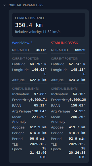 Orbital parameters showing semi-major axis, eccentricity, inclination, and period for both satellites.
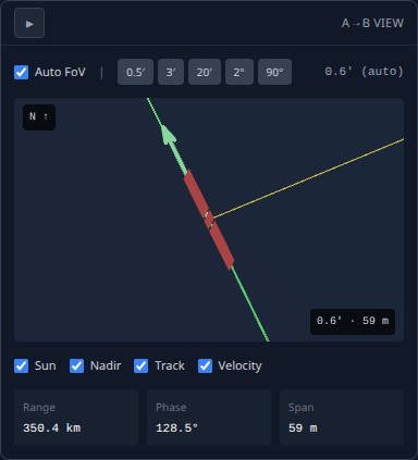 The A→B view shows what WorldView-3 “sees” looking at Starlink—useful for understanding imaging geometry.
It’s educational for understanding orbital mechanics: why some satellites get close frequently, why others never do, and how inclination, altitude, and RAAN affect conjunction patterns.
Conclusion
What started as a simple question—how quickly could they take this photo?—led me down an unexpected path.
I tried three approaches to reproduce the reported 241 km distance over Alaska. None succeeded. The closest I found was 204 km over the Atlantic, or 350 km near Kamchatka. Whether this gap reflects different ephemerides, a miles-vs-kilometers transcription error, or something else entirely, I can’t say for certain.
But the investigation was worth it. Building SatToSat taught me how satellite conjunctions actually work—the rhythm of close approaches, the physics of envelope periods, why some satellite pairs meet frequently while others never do. The scalloped patterns in the distance graphs aren’t just pretty; they encode real orbital mechanics.
Sometimes the most interesting answer to a question is discovering why you can’t answer it.
Discussion
The investigation details, analysis scripts, and envelope analysis are available in the SatToSat repository.